Bob talks
Bob Stuart, creator of MQA, talks in detail about this revolutionary British technology that sets a new standard in capturing, delivering and reproducing digital audio.
MQA CD: #1 Origami and the Last Mile
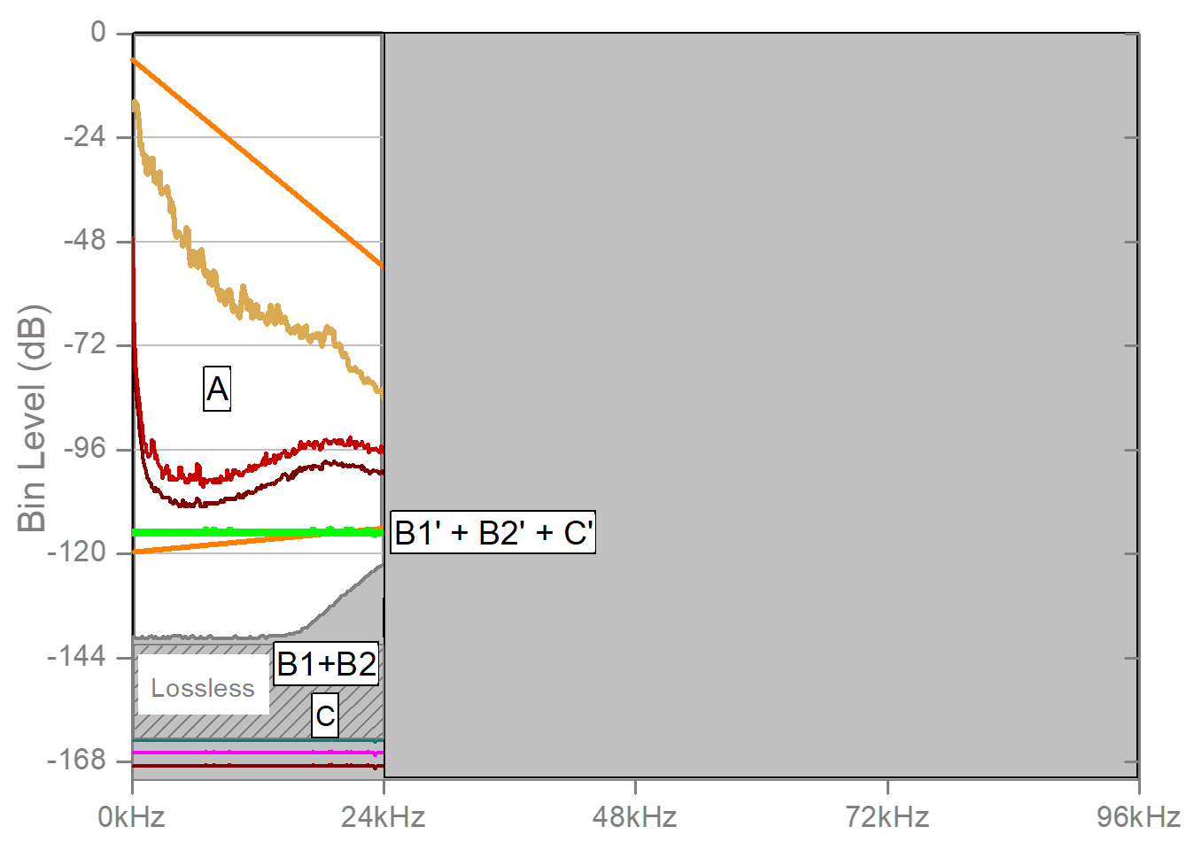
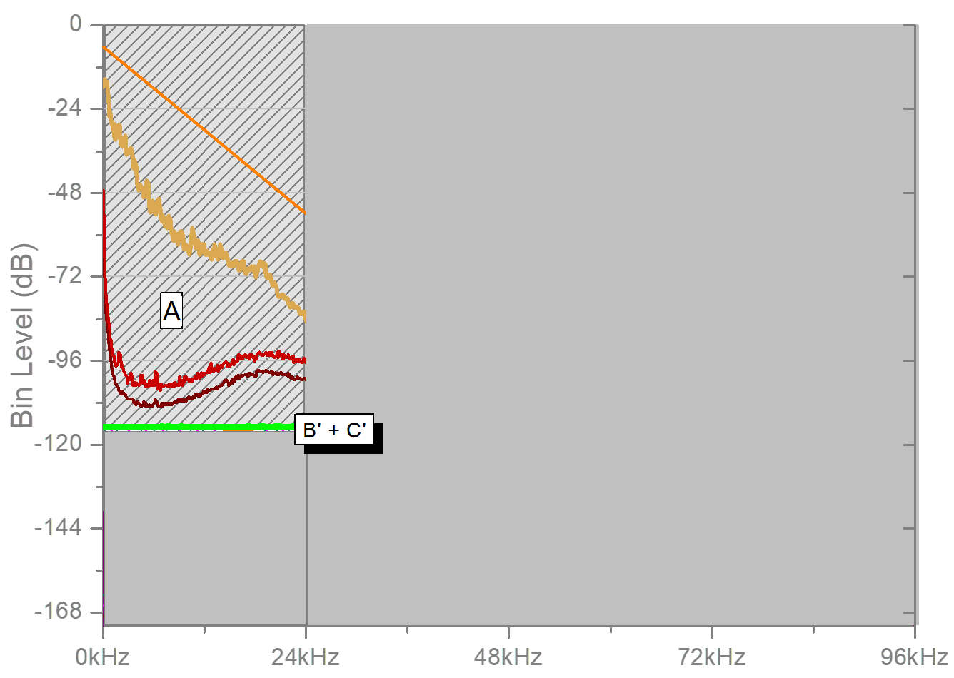
Once the recording has been ‘de-blurred’, MQA uses a process we call ‘Music Origami’ that focusses on maintaining the information in the orange triangle (plus a substantial safety margin), thereby making this large, high-resolution file both manageable, and compatible with any service or playback device. This section reviews the ‘origami’ used to make a single-speed (1s MQL) transmission file. As a first step, very high-frequency content (C) is ‘encapsulated’ and hidden away below the noise floor of B.
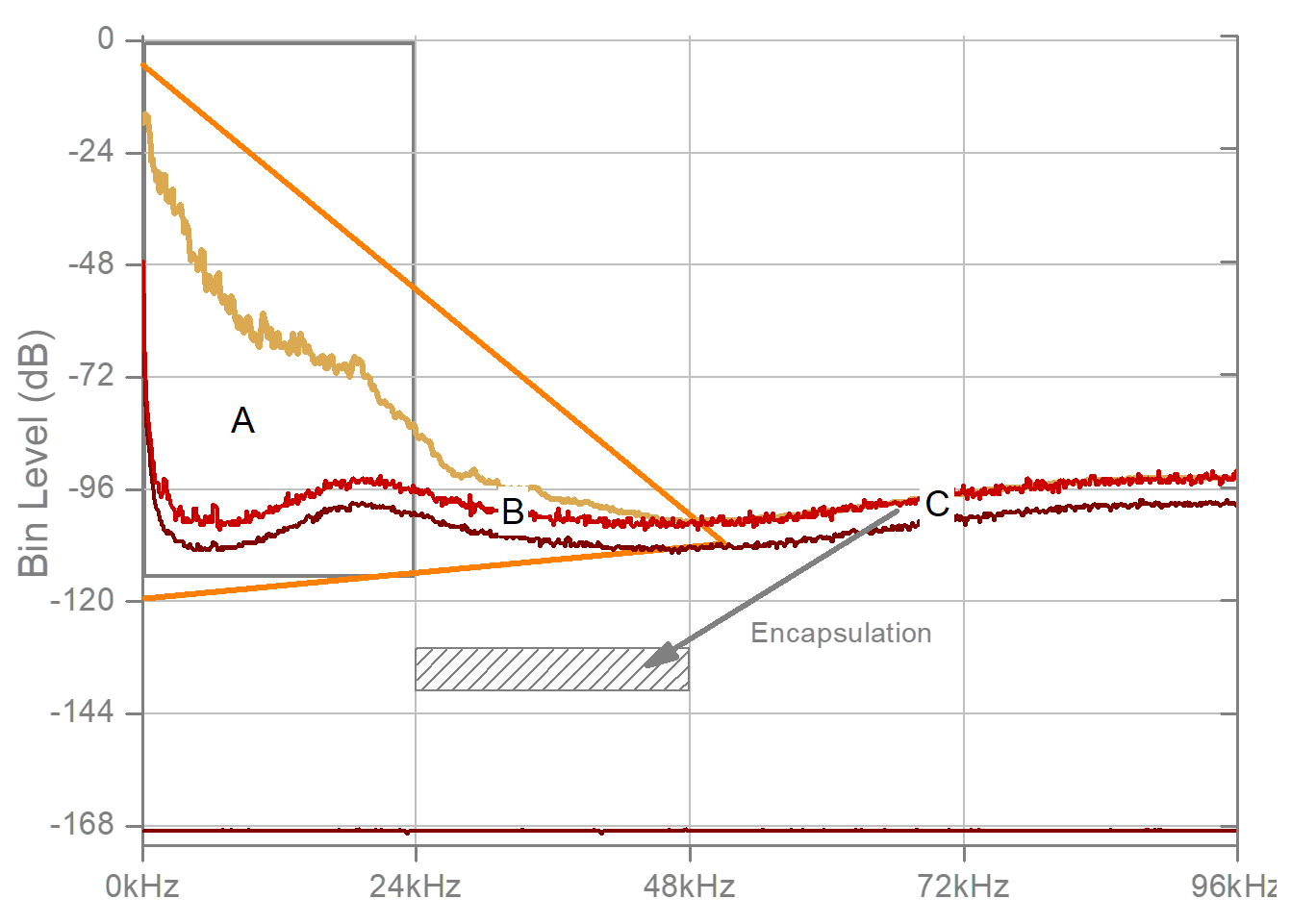 |
This Shannon information graph is sized to show the total spectrum capacity of 192kHz 24-bit PCM. The Grey rectangle shows the capacity of a CD. The gold curve is the peak level reached at any point throughout a music example. The red and brown lines show the maximum and average background noise – the sound we hear before the musicians start to play. All the salient music-related information exists inside the Orange triangle, which MQA protects very strictly. |
| Region A is the band of conventional audio information. | Region B, higher in frequency, manifests temporal microstructure in the sound. Region C carries noise consequential on the transmission sampling rate. |
 |
The next step is lossless burying of B and C well down in the noise below A. B is handled as two bands using custom lossless band-split and lossless processing and coding. At this stage, MQA signalling is added along with a small noise-shaped stream of information (Green line) that contains information about the recording, decoder instructions, as well as B and C. |
| The Green signal is completely removed by MQA decoders; but it is there so that we can hear more of the music when playback is limited to a 16-bit stream. | The coder for B uses an approximation (prediction) + a touch-up signal to make it lossless. The estimates of B1’ and B2’ can be buried within or below the green line (at the choice of the mastering engineer). |
 |
The next step is to fold this information into a small 48kHz 24-bit PCM file that you can hear wherever you play music today. If we don’t have a decoder this still sounds better than CD. This MQA file is low data rate – it is easy to stream and small to download. This encoded MQA file can also be previewed in the studio. We can play it on a Hi-Fi, a smartphone, a portable player, in the car, in a PC, on a Wi-Fi speaker or Bluetooth headphone. |
| This signal can be passed over a digital output to a downstream decoder. | Decoders can unwrap the Music to give us as much quality as the playback platform can support. The same file supports Studio quality playback and a smartphone! |
 |
Sometimes we might want to listen to MQA music on equipment that doesn’t support 24 bits – maybe only 16? Rather than throw away all the buried information, MQA carries a small data channel (shown in Green) which can contain the ‘B’ estimates, enabling significantly improved playback quality on, e.g. a CD, over ‘Airplay’, in-car, to certain WiFi speakers and similar scenarios. |
| If the target is a CD then specific coding is used to optimize the time-frequency balance and minimize the audibility of channel noise. | Of course, if your system handles 24 bits then the full file and dynamic range can be decoded. |
 |
The MQA ‘Core’ contains and protects all the music information in the Triangle – and more besides. It also contains region C and additional information – buried as noise, in noise, far below audibility. |
| A ‘Core’ decoder can unwrap back to this stage. In case the subsequent converters don’t go any faster, the MQA decoder has prepared this music for analogue replay. We can enjoy our music in 96 kHz 24-bit quality. | However, there is something special here. We can pass this 24-bit MQA Core signal on to another MQA device over USB, Lightning, S/PDIF, etc – and it is completely understood by a downstream MQA Decoder or MQA Renderer. |
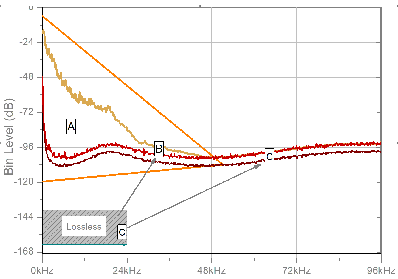 |
An MQA Decoder will continue to unfold as shown. Region C is reconstructed using buried instructions, which may have been pre-determined by the studio mastering engineer. At this step, the MQA decoder also handles compensation and filtering of the following D/A converter, which, depending on the model, may contain a cascade of signal processing, upsamplers or other forms of conversion and filtering. |
| This step in the decode process will be different for every product, in order to make the resulting analogue conform closely to the hierarchical target and to most accurately replicate what was approved in the studio. | The rendering stage can, on certain platforms, use cross-family rate conversion to maximise quality and minimize analogue blur. |
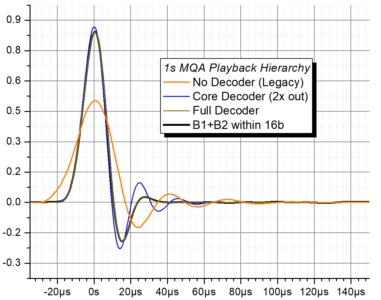 |
Showing the full system (analogue-to-analogue) average transmission kernel for the different decoding options shown in the previous two images. Olive is the full decoded result. When the transmission channel is limited to 16 bits, the decoder maintains good temporal performance, as the comparison between the olive and black curves show. Audio below 20 kHz is maintained at full resolution, while some precision is lost in the next octave. |
| If the final conversion to analogue is not using an MQA converter, the signals are preconditioned for a typical chip converter. The orange curve illustrates the input to the final converter if there is no decoder (‘Legacy mode’). | Blue shows the output of the ‘first unfold’ Core decoder at 2x speed. The orange and blue curves show the input to a DAC, not the analogue output. |
| |
Shows the Fourier transforms of the kernel responses in the previous image.
|
Index
MQA CD: #1 Origami and the Last Mile